Comparison dissolution profile analysis is a critical part of pharmaceutical formulation development and regulatory submissions. It helps determine whether the dissolution behavior of a test product matches that of a reference formulation.
Exploratory Methods for Comparison Dissolution Profile Analysis
Plotting the mean dissolution profile data for each formulation with error bars that extend to two standard errors at each dissolution time point is one way to visually represent the data. For instance, if the error bars at each dissolving time point do not overlap, the dissolution profiles for two formulations test (T) and reference (R) may be said to differ considerably from one another. This is because each dissolution time point’s error bars can be thought of as around 95% confidence intervals.
A numerical summary of the dissolution profile data can be used in addition to the graphical overview. Presenting the mean and standard deviation of the dissolve data for the test and reference formulations at each dissolution time point makes this feasible. A 95% confidence interval (the standard t-interval) for the variations in the mean dissolution profiles at each dissolution time point may be shown alongside the difference between the mean dissolution profiles. The difference at a particular dissolution time point is deemed to be significantly different at the 5% significance level if the 95% confidence interval for the mean difference does not contain zero.
Appropriate graphical and numerical techniques can also be utilized to represent the data in IR formulations where dissolution data are acquired at a single time point. Plotting the dissolution measurements for the test formulation next to those for the reference formulation allows for a visual representation of the data. With the exception of the fact that there will only be one dissolution time point at which to summarize the data, the data may be quantitatively summarized as previously mentioned for dissolution profile data. This exploratory data analysis may be deemed inadequate in several ways and is not meant to be exhaustive.
- Because the error bars for the two formulations might only overlap at certain time intervals, it could be challenging to draw a firm conclusion that the dissolution profiles for the two formulations differ. The numerical summary is subject to the same issue; that is, zero may appear in the 95% confidence interval for the difference between the mean test and reference formulations at some time points but not at others.
- The graphical representation of the mean dissolution profiles may appear overly cluttered if there are too many formulations to compare, especially with error bars at each dissolving time point. As a result, the dissolution data’s graphical plot could be challenging to understand. In a similar vein, if there were more than two formulations to compare, the numerical summary table would likewise grow significantly. This is due to the fact that each pair of formulations to be compared would have columns for the difference and the matching 95% confidence range.
Mathematical comparison methods
We describe two mathematical techniques for comparing dissolution profiles. Moore and Flanner characterized the first of these, whereas Rescigno described the second. A “difference factor” (equation 1) and a “similarity factor” (equation 2), sometimes referred to as the f2 equation, are two equations described by Moore and Flanner. The FDA dissolution guidance recommends using similarity factor (f2) for comparing dissolution profiles under appropriate conditions. These are the equations:
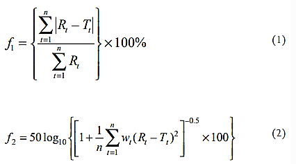
Where n is the number of dissolution time points, Rt and Tt are the reference and test dissolution values (mean of at least 12 dosage units1,2) at time t, and wt is an optional weighting factor.
The f1 equation is the sum of the absolute values of the vertical distances between the test and reference mean values, i.e. |Rt 2Tt | at each dissolution time point, expressed as a percentage of the sum of the mean fractions released from the reference formulation at each time point.
The average of the squared vertical distances between the test and reference mean dissolution values at each dissolution time point is transformed logarithmically to create the f2 equation, which is then multiplied by the proper weighting, wt (Rt 2Tt)2. The purpose of the weights, wt, is to give some dissolution time points greater weight than others. wt may be set to one at each time point if weighting time points is inappropriate. The f2 equation accepts values less than 100 as a result of the transformation. When the test and reference mean profiles are the same, the value of f2 is 100. In theory, it approaches minus infinity as ̩wt (Rt 2Tt)2 approaches infinity. In actuality, though, the maximum separation between mean dissolution profiles at any given time point cannot be greater than 100%; otherwise, the value of f2 will be nearly negative.
- The main advantages of the f1 and f2 equations are that they are easy to compute and they provide a single number to describe the comparison of dissolution profile data. However, there are disadvantages.
- The FDA suggests that the f2 equation should be applied when the within-batch variance, as measured by the coefficient of variation, is less than 15% (Ref. 1). The f1 and f2 equations do not account for the variability or correlation structure in the data.This implies that some research on the f2 equation may have been done to ascertain how data variability affects the method’s characteristics.
- The amount of dissolution time points used has an impact on the values of f1 and f2. • The disparities between the two mean profiles do not alter if the test and reference formulations are switched, but f2 does.
- It’s unclear what criteria are used to determine whether dissolution profiles differ or are similar.
Statistical/modelling methods
Statistical methods, unlike the mathematical methods described, go some way towards taking the statistical properties (variability and correlation structure) of the dissolution profile data into account in the comparison. These methods will be discussed under the following headings:
- One- and two-way analysis of variance (ANOVA) methods;
- Mixed effects model/multivariate methods;
- Modelling-based methods;
- Chow and Ki’s method.
One- and two-way analysis of variance (ANOVA) methods
None of the FDA advisory documents address these ANOVA techniques. The mean dissolution data at each dissolution time point are statistically compared separately using one-way analysis of variance techniques.When comparing the dissolution profile data for two formulations, the one-way analysis of variance is equal to a t-test. This method of comparing dissolution profile data ignores the correlation between the dissolution time points, treating each time point as if it were independent of the others, which is obviously not the case, even though it accounts for the variability in the dissolution profile data at each time point. Additionally, the total risk of mistakenly determining that the mean dissolution profiles differ (the type I error) is significantly greater than the nominal 5% threshold, which is a well-known result of carrying out multiple comparisons (t-tests or one-way analyses of variance). With the exception of IR data at a single dissolution time point, where the one-way analysis of variance approach is appropriate, the use of these ANOVA methods is not advised due to the previously described restrictions.
Mixed effects model/multivariate methods
Mauger et al. tested if the real dissolution mean profiles for each formulation are parallel (i.e., do the profiles have the same shape) using the mixed effects model. and if the actual mean profiles of dissolution are at the same level. Fixed and random effects are combined in the mixed effects model. Formulation is the fixed effect in the context of comparing dissolution profile data; if test and reference formulations are being compared, there will only be two levels. Dosage units, which have as many varied values for each formulation as there are dosage units in the batch, are the random effect in the model. A number of dose units are chosen at random for dissolving testing for a particular formulation. Because conclusions regarding the formulation under test will be drawn from the dosage units chosen at random for the dissolving experiment, the dosage unit effect is therefore a random effect.
The coincidence hypothesis mentioned earlier can also be tested using a multivariate technique called Hotelling’s T2 test. Although it is less effective than the mixed effects model when the data’s covariance structure is compound symmetric, this does not make any limiting assumptions about the data’s covariance structure. Tsong et al. present a multivariate approach that measures the difference between mean dissolution profiles using the Mahalanobis distance, which accounts for variability and correlation structure. This approach can be viewed as a multivariate equivalent of the two-sided t-test method used to determine average bioequivalency.
Modelling-based methods
The approach, which is based on mechanistic models that explain the dissolving events described by Crowder, compares data for various formulations using repeated measures regression analysis approaches. These data show how long it takes for different dosage unit fractions to dissolve (the method can also be used to analyze data that show the fraction of the dosage unit dissolved at predefined times). Because it employs significant mechanistic models and considers the covariance structure in the statistical comparison of the data, this method is thought to be better than other modeling-based methods. The adequacy of the mechanistic models employed can be assessed by diagnostic tests. However, this method may be difficult to implement in practice because it may be difficult to analyse the data through the use of conventional statistical packages.
The FDA solely takes into account the modeling-based approach proposed by Sathe et al.1. However, it’s uncertain in what circumstances it should be applied, and it’s unknown how much these modeling-based techniques are used. The approach outlined by Crowder26 is thought to be the best of the existing approaches since it combines repeated-measures regression analysis, which considers the correlation structure of the data, with mechanistic models to characterize the data. However, utilizing normal statistical tools to put this strategy into practice could be challenging.
Chow and Ki’s method
A technique for comparing dissolution profile data that can be thought of as comparable to that used in evaluating the average bioequivalency of two drug formulations is described by Chow and Ki27No FDA advisory paper mentions this technique, and it’s unclear how widely it’s employed. If the ratio of the mean bioavailability parameters [area under the curve (AUC), Cmax, etc.] falls between the 80–125% bioequivalence criteria with 90% confidence, then the test and reference formulations are bioequivalent in average bioavailability. Q, the intended mean dissolution rate of a medicine as stated in the USP/NF, is used to calculate the equivalency standards for similarity between dissolution profiles at each dissolution time point proposed by Chow and Ki. The dissolution statistics for the two formulations are deemed “locally similar” at a given time point if the ratio of the mean dissolution rates for the test and reference formulations is within the equivalency limits at that time point with a particular degree of confidence, such as 90%. If the two formulations’ dissolution profiles are comparable at every dissolution time point, they are said to be “globally similar.”
The ratio of the test and reference percentages released at each time point is described using an autoregressive-time series model, which accounts for the correlation between subsequent dissolution time points. Implementing this method for comparing dissolution profile data is not too difficult. Nevertheless, Type I error (the likelihood of determining that the dissolution profiles are considerably different when they are similar) and Power (the likelihood of identifying a significant difference between dissolution profiles when they are genuinely different) are currently unknown.
Need Support with Comparative Dissolution Profile Studies?
- A robust Comparative Dissolution Profile study can make the difference between a smooth regulatory journey and unnecessary delays.
- Partner with Regcure Pharma to ensure your pharmaceutical formulations meet global regulatory expectations with accuracy, consistency, and scientific credibility.
- If you need expert support in dissolution profile comparison, BE studies, or regulatory dossier preparation, our regulatory experts are ready to assist.
- 📧 Email: info@regcurepharma.com
- 🌐 Website: www.regcurepharma.com
- 📞 Contact: +91-8799045524